[Super Resolution] Using Hugging Face Diffusers

출처 : https://pyimagesearch.com/2024/06/03/sharpen-your-vision-super-resolution-of-cctv-images-using-hugging-face-diffusers/ 의 글을 한글 번역과 저의 의견 및 코드 수정을 거친 Post입니다.

Sharpen Your Vision: Super-Resolution of CCTV Images Using Hugging Face Diffusers - PyImageSearch

디퓨전 모델: 이미지 생성의 새로운 패러다임

디퓨전 모델(Diffusion Models)은 최근 몇 년 사이 컴퓨터 비전 분야에서 가장 주목받는 생성 모델 중 하나로 부상했습니다. 특히 unconditional 및 conditional 이미지 생성 태스크에서 놀라운 성능을 보여주고 있죠.

 

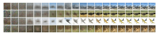
DDPM: 디퓨전 모델의 시작 The first iteration of what we now call a standard diffusion model was the Denoising Diffusion Probabilistic Model (DDPM).

 

This model introduced a simple yet effective process for image generation.

 

• DDPM의 핵심 아이디어는 다음과 같습니다:
  1. 노이즈 추가 (Add Noise)
     • 초기 이미지에 점진적으로 가우시안 노이즈를 추가합니다.
     • 이 과정은 여러 단계에 걸쳐 이루어지며, 최종적으로는 원본 이미지의 모든 정보가 사라집니다.
  2. 노이즈 제거 학습 (Learn to Remove Noise)
     • UNet과 같은 denoising 모델을 사용하여 각 타임스텝에서 노이즈가 제거된 이미지를 예측합니다.
     • 이 과정은 노이즈를 추가한 횟수만큼 반복됩니다.
  3. 추론 (Inference)
     • 학습된 denoising 네트워크를 사용하여 랜덤 노이즈 이미지로부터 시작해 점진적으로 현실적인 이미지를 생성합니다.
  디퓨전 모델의 발전 Since the introduction of DDPM, various improvements and variations have been proposed:
  • 노이즈 예측 vs 이미지 예측: 일부 모델은 추가된 노이즈를 직접 예측하고 이를 빼는 방식을 사용하는 반면, 다른 모델들은 노이즈가 제거된 이미지를 직접 예측하기도 합니다.
  • 샘플링 속도 개선: 초기 모델들은 샘플링에 수백 단계가 필요했지만, 최근 연구들은 이를 크게 단축시키는 데 성공했습니다.
  • Conditional Generation: Text-to-Image 모델들과 같이 조건부 생성을 가능하게 하는 기술들이 개발되었습니다.
  디퓨전 모델은 그 우수한 성능과 유연성으로 인해 계속해서 발전하고 있으며, 앞으로도 컴퓨터 비전 분야에서 중요한 역할을 할 것으로 기대됩니다.

The progressive denoising process to generate images (source:   Ho, Jain, and Abbeel, 2020 ).

디퓨전 모델의 진화: 잠재 디퓨전 모델 (Latent Diffusion Model)

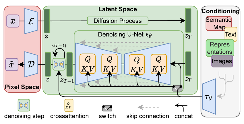
디퓨전 모델의 발전 과정에서 Rombach 등(2022)이 제안한 잠재 디퓨전 모델(Latent Diffusion Model, LDM)은 획기적인 발전을 이루었습니다.

 

이 모델은 이미지 처리 방식을 혁신하고 텍스트 프롬프트를 통한 생성 제어 기술을 도입했습니다.

LDM의 주요 특징

LDM은 다음과 같은 접근 방식을 구현합니다:

1. 잠재 공간 인코딩
   • 이미지를 잠재 공간 표현으로 인코딩합니다.
   • 이 과정은 대규모 이미지 데이터로 사전 학습된 신경망 인코더를 사용합니다.
2. 잠재 공간에서의 노이즈 추가
   • 노이즈 추가 과정이 잠재 공간 표현에서 수행됩니다.
   • 이는 작업의 효율성을 크게 향상하며, 이미지 크기와 무관하게 연산량을 줄입니다.
3. 디노이지 네트워크
   • 노이즈 제거 과정을 역전시켜 깨끗한 이미지로 디코딩될 잠재 표현을 예측합니다.
   • 노이즈나 이미지 자체를 직접 예측하는 대신 이 방식을 사용합니다.
4. 텍스트 조건부 생성 (선택적)
   • 텍스트 프롬프트를 사용하여 이미지 내용을 제어할 수 있습니다.
   • 텍스트 인코더를 통해 프롬프트를 처리하고 이를 디노이징 네트워크에 주입합니다.
5. 이미지 디코딩
   • 디노이징 후 최종 잠재 표현을 이미지 디코더에 통과시킵니다.
   • 이 디코더는 또 다른 신경망으로, 잠재 표현을 입력받아 원본보다 고해상도의 출력을 생성합니다.

LDM의 의의

LDM은 기존 디퓨전 모델의 한계를 극복하고 효율성을 크게 향상했습니다. 특히 텍스트 프롬프트를 통한 이미지 생성 제어 기능은 다양한 응용 분야에서 큰 주목을 받고 있습니다. 초해상도(super-resolution) 작업에서는 텍스트 조건부 생성 기능을 사용하지 않지만, LDM의 기본 구조를 활용하여 효과적인 이미지 품질 향상이 가능합니다.

The Latent Diffusion Model architecture (source:   Rombach et al., 2022 ).

 

 

본 튜토리얼을 진행하기 위해 필요한 package 등을 pip를 통해 다운로드하여 줍니다.

 

 pip install roboflow diffusers accelerate 
 huggingface_hub peft transformers datasets safetensors 
 scipy bitsandbytes xformers -qqq

• Diffusers for model loading and inference
• Roboflow for Dataset loading
• Torch for Tensor manipulation
• Matplotlib for Image plotting
• Datasets for Dataset registration and manipulation
• Numpy for Array manipulation

import os
import torch
import numpy as np
from roboflow import Roboflow
import matplotlib.pyplot as plt
from datasets import load_dataset
from diffusers import LDMSuperResolutionPipeline
from mpl_toolkits.axes_grid1.inset_locator import mark_inset, zoomed_inset_axes

 

필요한 변수들을 저장해 주겠습니다

device :  GPU, CPU등 하드웨어 가속기를 설정해 줍니다.

 

model_id : Hugging Face Hub에서 사용 가능한 Model을 선언해 줍니다.

num_samples : 나중에 시각화를 위해 보여줄 이미지 갯수 입니다.

 

device = "cuda" if torch.cuda.is_available() else "cpu"
model_id = "CompVis/ldm-super-resolution-4x-openimages"
num_samples = 3

 

Roboflow를 통해 data를 download 해줍니다. (optional, 데이터가 있으시다면 필요 없는 부분입니다.) 

Roboflow(api_key = " ") <- 이 안에 roboflow 가입하시고 workspace 만든 다음에 settings 들어가시면 private API KEY를 알 수 있는데 그걸 그대로 copy 하면 됩니다,

private API key 복붙 하시면 됩니덩~

 

datasets : Hugging Face-compatible dataset representation (that is also compatible with the torch.utils.data.Dataset APIs).

 

rf = Roboflow(api_key="")
project = rf.workspace("combine-iixr2").project("retailshop-1gysu")
version = project.version(4)
dataset = version.download("yolov5")
dataset = load_dataset(
"imagefolder", 
data_dir="/content/RetailShop-4"
).shuffle(seed=42)

 

pipeline : Diffusers로 부터 import하고 model ID를 정해 줌으로고 나중에 infer로 사용할 weights를 저장합니다.

 

 

Ampere GPU이상의 하드웨어를 사용할 수 있는 환경이라면,  torch.bfloat16 datatype으로 바꿔서 효율적인 연산을 할 수 있습니다.

 

ldm_pipeline = LDMSuperResolutionPipeline.from_pretrained(
    model_id, torch_dtype=torch.float16
    # if using an Ampere-class GPU or above, use torch.bfloat16 for benefits
)
ldm_pipeline = ldm_pipeline.to(device)

 

We now define a runner function called 

pipe : original pipeline inference call을 감싸주고 원하는 결과(image)만 얻어내도록 합니다. 

 

def pipe(image):
    return ldm_pipeline(image, num_inference_steps=100, eta=1).images

모델과 데이터를 얻었으니 Super Resolution 초해상화 결과를 num_inference_step을 걸쳐 생성합니다.

 

res_originals = []
res_outputs = []
for idx in range(0, num_samples):
    item = dataset["train"][idx]
    res_image = pipe(item["image"])
    res_originals.append(item["image"])
    res_outputs.append(res_image)

 

다양한 plotting 예시를 keras.io에서 볼 수 있습니다. Super Resolution 역시 한눈에 보기 좋게 plotting 하는 방법을 아래 제시합니다.

A good plotting function is always important to understand the effects of our results. Taking some inspiration from this

awesome tutorial on Keras.io, we define our own plotting function that accepts the original and higher-resolution image and performs some zooming and nifty tricks to get an awesome visualization experience!

Keras documentation: Image Super-Resolution using an Efficient Sub-Pixel CNN

 

기존 posting의 plot_image_with_zoom코드의 경우 이미지의 절대사이즈를 활용하기 때문에 상대 사이즈로 dynamic 하게 받아올 수 있도록 수정한 코드입니다.

plt.rcParams["figure.figsize"] = (num_samples*5, 5)  # Adjust as needed
plt.rcParams["figure.dpi"] = 300
def plot_image_with_zoom2(original_img, res_img, zoom_factor=1.5, zoom_region_fraction=0.25):
    original_np_img = np.asarray(original_img)
    res_np_img = np.asarray(res_img).squeeze(0)
    
    # Normalize images to range [0, 1]
    original_np_img = original_np_img.astype("float32") / 255.0
    res_np_img = res_np_img.astype("float32") / 255.0
    
    # Get dimensions for original and superresolution images
    og_height, og_width, _ = original_np_img.shape
    sr_height, sr_width, _ = res_np_img.shape
    
    # Calculate the larger zoom region for the original image
    og_region_size = int(min(og_height, og_width) * zoom_region_fraction)
    og_x1, og_x2 = og_width // 2 - og_region_size // 2, og_width // 2 + og_region_size // 2
    og_y1, og_y2 = og_height // 2 - og_region_size // 2, og_height // 2 + og_region_size // 2
    
    # Calculate the larger zoom region for the superresolution image
    sr_region_size = int(min(sr_height, sr_width) * zoom_region_fraction)
    sr_x1, sr_x2 = sr_width // 2 - sr_region_size // 2, sr_width // 2 + sr_region_size // 2
    sr_y1, sr_y2 = sr_height // 2 - sr_region_size // 2, sr_height // 2 + sr_region_size // 2
    
    # Adjust figure size dynamically
    fig, ax = plt.subplots(1, 2, figsize=(12, 6), dpi=200)
    
    # Display original and superresolution images
    ax[0].imshow(original_np_img)
    ax[0].axis('off')
    ax[0].set_title("Original Image")
    
    ax[1].imshow(res_np_img)
    ax[1].axis('off')
    ax[1].set_title("Super Resolution Result")
    
    # Create zoomed insets for original image
    original_axins = zoomed_inset_axes(ax[0], zoom_factor, loc=2)
    original_axins.imshow(original_np_img, origin="lower")
    
    # Create zoomed insets for superresolution image
    res_axins = zoomed_inset_axes(ax[1], zoom_factor, loc=2)
    res_axins.imshow(res_np_img, origin="lower")
    
    # Set zoom region limits for original image
    original_axins.set_xlim(og_x1, og_x2)
    original_axins.set_ylim(og_y1, og_y2)
    
    # Set zoom region limits for superresolution image
    res_axins.set_xlim(sr_x1, sr_x2)
    res_axins.set_ylim(sr_y1, sr_y2)
    
    # Remove ticks from zoomed insets
    original_axins.set_xticks([])
    original_axins.set_yticks([])
    res_axins.set_xticks([])
    res_axins.set_yticks([])
    
    # Draw rectangles around zoomed regions
    mark_inset(ax[0], original_axins, loc1=1, loc2=3, fc="none", ec="blue")
    mark_inset(ax[1], res_axins, loc1=1, loc2=3, fc="none", ec="blue")
    # plt.axis('off')    
    plt.show()

 

찍어봅시다.

plot_image_with_zoom(res_originals[0], res_outputs[0])
# Iterate over each of the samples to get the result

 

오늘은 간단하게 DDPM을 활용한 Super Resolution 예시를 실행해 봤습니다.

 

보기 좋은 Plotting idea를 얻은 것만으로도 큰 수확입니다,