K-lane LLDN(Lidar Lane Detection Network )
1. 역사
- CLDN : 카메라 기반 차선 감지는 조명 조건에서 상당한 성능 문제가 존재하지만 라이다는 야간, 빛 등 다양한 조명 조건에 강함
- 카메라 기반 방법은 자차로부터의 거리에 따라 두께가 감소하여 동일한 소실점을 향하게 되어 차선 끝에 왜곡 문제 존재
- LLDN : 초기 라이다 기반 차선 감지는 차선 표시를 식별하기 위해 강도 또는 반사율 임계값 설정에 의존하였지만 사전 정의된 임계값에만 한정되어 다양한 조로 환경 조건에 부합하지 않았음
2. LLDN GFC(Lidar Lane Detection Networks utilizing Global Feature Correlator)
- LLDN-GFC(Lidar lane detection networks utilizing global feature correlator) f1 score 82.1%
- LLDN-GFC는 포인트 클라우드 상의 차선의 Spatial Characteristics을 활용
- spatial characteristics of lane : 희소하고, 얇으며, 포인트 클라우드의 전체 지면을 따라 늘어서 있음
- LLDN-GFC는 차선을 위한 Global Feature Correlator를 수행하기 위해 Transformer와 Mixer 블록 기반으로 구현
- 요약
- 점군 → 2D(BEV) 변환: 3D 라이다 점군을 Bird’s Eye View(BEV) 형태로 투영하여 2D 특징 맵을 생성
- BEV 패치 임베딩: BEV 특징 맵을 고정 크기의 패치들로 나누고 각 패치를 벡터 형태로 변환(임베딩)
- 패치 간 상관관계 학습: GFC(Transformer 또는 MLP-Mixer)를 통해 패치들 간의 전역적 관계 학습
- BEV 형태의 맵으로 재구성: 학습된 패치 시퀀스를 다시 원래 BEV 특징 맵 형태로 변환
- 최종 특징 맵 형성: Detection Head를 통해 픽셀 단위로 차선 분류 및 신뢰도 맵을 생성
2.1 BEV Encoder
- 두 가지 주요 BEV 인코더(용도에 따라 적절한 인코더 선택)
- BEV 인코더는 3D 포인트 클라우드를 pseudo-BEV 2D 이미지로 투영하고 처리하여 2D BEV 특징 맵을 생성
- Point Projector
- 논문에서는 포인트 클라우드를 xy-평면에 투영하고 CNN을 사용하여 2D BEV 특징 맵을 생성
- 3개의 추가 정보(z좌표, 강도, 반사도-(z, intensity, and reflectivity))를 사용하여 생성된 pseudo-BEV 2D 이미지의 3개 채널을 생성
- 실시간 속도를 유지하면서 고해상도 차선 정보를 유지하기 위해 유사한 BEV 이미지 입력의 1/8² 이 되는 특징 맵을 출력하는 CNN의 깊이까지만 사용
- BEV 이미지는 라이다 포인트 클라우드의 x, y 좌표를 평면에 배치하고 z좌표와 강도, 반사도(z, intensity, and reflectivity)의 특성을 채널 값으로 사용하여 2D 이미지처럼 표현한 데이터 구조
- 다수의 휴리스틱 경로 계획 알고리즘과 엔드투엔드 자율 주행 알고리즘[2]은 2D BEV 이미지 상의 차선 정보를 필요로 함
- Pillar Encoder
- Point Pillars 기반의 인코더 상대적으로 작은 네트워크 크기를 가짐
- Point Projector에비해 상대적으로 작은 네트워크 크기를 가진 저 연산 2D BEV Encoder
- CNN 기반 Point Projector 보다 낮은 성능을 보이며 더 빠른 추론 속도를 가짐
- 논문에서 설명하는 방식은 수평면의 각 격자에 포인트 클라우드를 정렬하여 Ng×Nc×Np 크기의 적층된 필러를 생성
- (Ng는 격자의 총 수, Nc는 포인트 특징 구성요소, Np는 격자에 존재하는 최대 포인트 수)
2.2 GFC(Global Feature Correlator)
- 도로 위 차선은 얇고 전체 포인트 클라우드를 따라 늘어서 있어 소수의 픽셀만 차지해 데이터 내 차선 정보는 희소함
- 얇은 특성과 희소성으로 인해 고해상도에서 특징 추출을 수행 필요
- Feature Correlator는 BEV 특징 맵 내의 멀리 떨어진 grid 간의 상관관계를 고려 필수
- GFC는 patch 단위의 self-attention network를 활용하여 고해상도에서 특징들의 전역적 상관관계 연산 진행
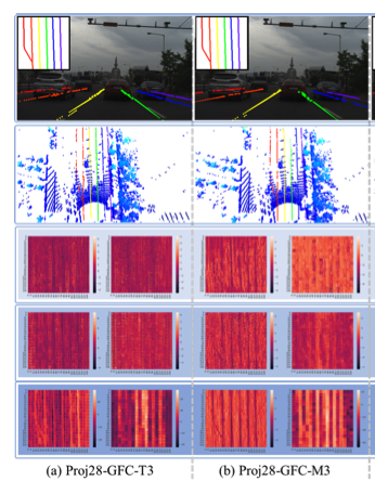
- GFC-T (transformer 기반)
- 글로벌 상관 관계를 계산하기 위해 트랜스포머 블록 사용
- 성능이 더 좋지만 계산 비용이 더 높음
- GFC-M (MLP-Mixer 기반)
- 글로벌 상관 관계를 위해 Mixer 블록 사용
- 계산 비용이 낮지만 성능이 약간 떨어짐
- GFC-T (transformer 기반)
3. Detection Head
- GFC에서 추출된 특징 맵을 받아 최종 차선 예측
- 두 개의 Segmentation Head로 구성
- Detection Head 설계 시, 차선 감지 문제를 다중 클래스 분할 문제로 다루어 각 픽셀에 클래스와 신뢰도 점수가 할당되도록 진행
- LLDN-GFC의 Detection Head는 중간에 비선형 활성화 함수가 있는 두 층의 shared-MLP 시퀀스로 구성되어 있음
- Confidence Head
- 각 픽셀이 차선에 속하는지 아닌지를 예측하는 Binary Segmentation로 차선 픽셀과 배경 구분 수행
- 출력 맵 : Hbev * Wbev * 1 크기의 Confidence map
- Confidence map : 각 픽셀의 차선 여부 확률
- 활용 예시 : 차선이 끊어진 경우에도 주변 픽셀을 보고 연속성 추론 가능
- 활성화 함수 : sigmoid 함수를 통해 0~1 사이의 확률 값 생성
- 손실 함수 : Soft Dice Loss 손실 함수 사용
- 클래스 불균형 문제 처리 적합
- 배경보다 차선 샘플이 훨씬 적은 문제 해결
- Classification Head
- 차선 클래스를 예측(예시:자차 차선, 1차선, 2차선 등)하는 Multi-Class Classification 문제
- 출력 맵 : Hbev * Wbev * Ncls 크기의 Classification map (Ncls는 클래스 수)
- Classification map : 각 픽셀이 속한 차선 클래스의 확률
- 활용 예시 : 다차선 도로에서 개별 차선을 구분하여 검출
- softmax 함수를 통해 클래스별 확률값 생성
- Grid-wise Cross-Entropy Loss 손실 함수 사용
- 다중 클래스 분류 문제 자주 사용
- 네트워크가 학습 중에 올바른 차선 클래스의 확률을 최대화하도록 유도
- Confidence Head
1. History
1.1 Lane Detection Networks for Camera
CLDNs have some inherent problems. In the CULane benchmark, most of the CLDNs show significant performance drop (about 20%) for night time and dazzling light conditions from their daytime performance
1.2 Early Lane Detection Techniques for Lidar
in early studies, lane points are detected by thresholding the measured intensity (or reflectivity). However, these heuristic techniques rely on pre-defined thresholding parameters, and, therefore, it is not very adaptive to different environments.
1.3 Lane Detection Networks for Lidar.
LLDN that combines 2D BEV images developed with the Lidar point cloud and the front camera image for lane detection.
CNN-based LLDN that uses BEV images from point clouds to detect ego-lanes, and tests the network in an uncrowded highway.
1.4 Thus
We observe that the CNN-based LLDNs are not suitable for detecting lane lines in Lidar point cloud. For example, lane lines on the front view image have decreasing thickness with the distance from the ego vehicle and are heading to the same vanishing point (on a straight road), whereas lane lines in a BEV image have a constant thickness and stretch long in parallel over the entire BEV image.
2. Engines
backbone model = LLDN-GFC(Lidar lane detection networks utilizing global feature correlator) f1 score 82.1%
LLDN-GFC exploits the spatial characteristics of lane lines on the point cloud, which are sparse, thin, and stretched along the entire ground plane of the point cloud.
The proposed LLDN-GFC can be implemented with Transformer [5] and Mixer [29] blocks to perform an effective global feature correlation for lane lines.
1. 점군 → 2D(BEV) 변환: 3D 라이다 점군을 Bird’s Eye View(BEV) 형태로 투영하여 2D 특징 맵을 생성.
2. BEV 패치 임베딩: BEV 특징 맵을 고정 크기의 패치들로 나누고, 각 패치를 벡터 형태로 변환(임베딩).
3. 패치 간 상관관계 학습: GFC(Transformer 또는 MLP-Mixer)를 통해 패치들 간의 전역적 관계를 학습.
4. BEV 형태의 맵으로 재구성: 학습된 패치 시퀀스를 다시 원래 BEV 특징 맵 형태로 변환.
5. 최종 특징 맵 형성: Detection Head를 통해 픽셀 단위로 차선 분류 및 신뢰도 맵을 생성.

2.1 BEV Encoder
The BEV encoder projects a 3D point cloud into a 2D pseudo-image and process it further to produce a 2D BEV feature map.
2.1.1 Point Projector
BEV encoder projects 3D point cloud into a horizontal plane to produce 2D pseudo-BEV image. A large number of heuristic path planning algorithms, such as A* [7], RRT* [10], and End-to-End autonomous driv- ing algorithms [2] require lane lines on 2D BEV images.

point projector projects point clouds into the xy-horizontal plane and produces a BEV feature map using CNN. In this case, three additional information (z, intensity, and reflectivity) other than x and y of the point cloud is used to generate three channels of the produced pseudo-BEV image.
In order to maintain both high-resolution lane information and real-time speed, we design a ResNet-based CNN to output a feature map that is 1/82 of the pseudo-image input.
2.1.2 Pillar encoder
pillar encoder is an alternative for low computational 2D BEV encoder.
Pillar encoder has slightly lower performance but faster inference speed than the CNN-based point projector.
2.2 Global Feature Correlator (GFC) AS BACKBONE
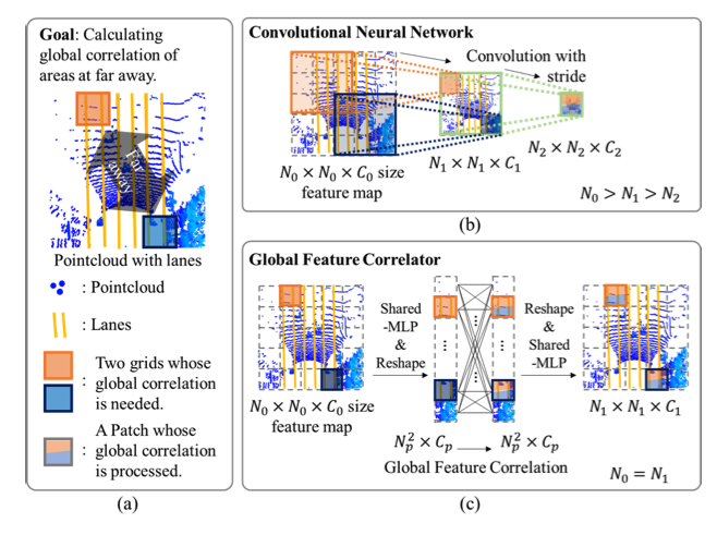
lane lines on the road are thin, stretched along the entire point cloud, and only occupy a small number of pixels (i.e., sparse). Due to such thinness and sparsity, it is necessary to perform feature extraction in high resolution. In addition, the feature extractor should consider the correlation between distant grids within the BEV feature map.
So, GFC calculate global correlations of the features in high resolution by utilizing patch-wise self -attention networks.
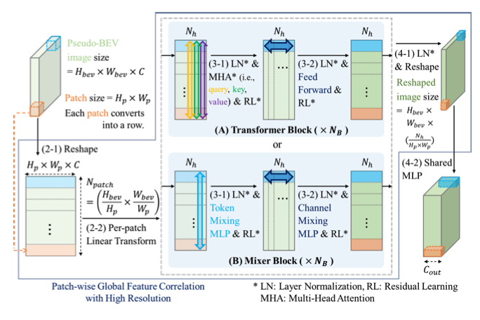
2.2.1 GFC-T(GFC-Transformer blocks)
2.2.2. GFC-M(GFC-Mixer blocks)
2.3 Detection Head and Loss Function
To design the detection head, we formulize the lane detection problem as a multi-class segmentation problem, where each pixel is as-signed a class and a confidence score.
The LLDN-GFC detection head consists of two segmentation heads, each of which consists of a sequence of two-layer shared-MLP with a non-linear activation in-between.
'On Going > Point Cloud Data' 카테고리의 다른 글
| [pcd] 도로 포인트클라우드를 평면으로 정렬하는 4가지 방법: 딥러닝 전처리를 위한 접근(3. DTM기반 CSF) (0) | 2025.04.14 |
|---|---|
| [pcd] 도로 포인트클라우드를 평면으로 정렬하는 4가지 방법: 딥러닝 전처리를 위한 접근(2. Moving Least Squares) (0) | 2025.04.14 |
| [pcd] 도로 포인트클라우드를 평면으로 정렬하는 4가지 방법: 딥러닝 전처리를 위한 접근(1. RANSAC) (0) | 2025.04.14 |
| [PCD] Point Transformer V3(PTv3) 논문리뷰 (0) | 2025.03.17 |
| [PCD] start (0) | 2025.03.12 |
댓글